
Browser access was lost. Refresh the app to start again. Earlier recordings cannot be restored in a new browser session.
My recordings
These recordings are available in this browser. Download the results you want to keep before expiry.
Find suitable
cutoff frequencies.
Upload a C3D to compare marker and ground reaction force cutoff frequencies. Get suggested settings, supporting plots and an explanation of their limitations.
Get a marker cutoff suggestion from movement data.
Check marker and force settings together.
With supported calibration, compare how filter settings affect joint moments.
Your conclusion
Analyse a recording to compare two provisional cutoff methods on the same selected upload data.
- 1 Upload
- 2 Review
- 3 Results
Upload your C3D
Choose a continuous C3D and review its preprocessing, channels and units. Use walking/running presets for gait, or General movement for marker diagnostics of other movements, including landing. General mode does not support force or joint-moment recommendations.
What to prepare before uploading
- Marker diagnostics: a C3D with physical marker coordinates and stated length units. Point labels may also contain computed outputs: exclude those. Channels with missing frames are excluded from this signal screen; it does not fill gaps.
- Force checks: calibrated force-platform signals in newtons (N), known global vertical axis and sign, checked synchronization, and at least two complete interior contacts. Upload the continuous recording, rather than separately cut stance clips.
- Experimental joint moments: the same participant’s static C3D, measured mass (kg) and height (m), and the supported physical marker protocol below. Ordinary marker names or mass and height alone do not provide a calibration.
Public examples include downloaded recordings and, where supported, participant calibration. Review the confirmations yourself: selecting an example does not confirm its validity.
Checking how this analysis server stores uploaded files…
Run a real recording to explore your own settings. For an immediate explanation with saved measurements, choose “Public-data examples” above.
Test another downloaded recording
Other participants and running speeds. Each file is checked independently; available joint-moment support depends on its calibration.
Recording review
Current-run figures and downloads
The two recommendations above are calculated from this upload and the same selected marker coordinates. Current figures show both live signal methods. Teal denotes ACF, orange Winter, and gray raw force or reference construction.
Tested frequencies and analysis support
Marker evidence · both live methods
Left: ACF residual score (dimensionless) versus cutoff (Hz); lower score is preferred. Middle: one named coordinate’s removed-motion RMS (mm), tail fit, zero-frequency intercept, and its crossing. Right: valid coordinate crossings with the Winter median candidate. The Winter median is not a crossing of a median residual curve. Dashed candidate lines use Hz. Both diagnostics trim 1 s at each end; the marker summary CSV uses its separately declared comparison guard. Removed motion can include signal and noise; these panels do not establish accuracy.
Force evidence · exact matched candidate settings
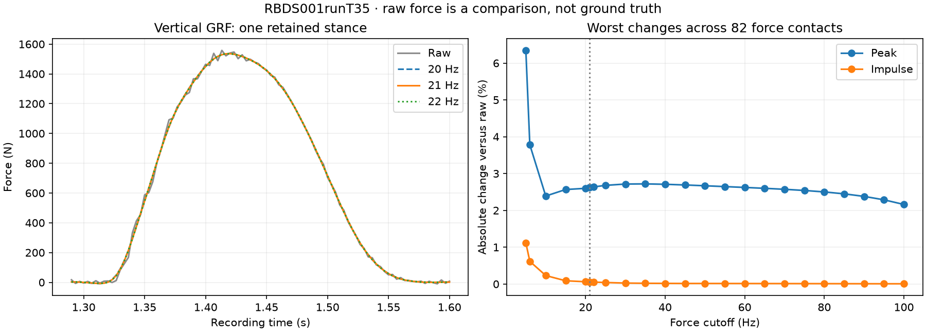
Compare raw and filtered vertical force (N) over one fixed contact. Below, peak and impulse changes (%) are shown separately with labeled review limits. Smaller changes mean closer agreement with the recorded raw signal, not greater accuracy. Impulse is the area under the force curve (N·s). The peak and impulse charts use different horizontal scales; compare their percentage labels.
Other moment settings, full recording and eligibility details
Experimental joint moments at selected settings
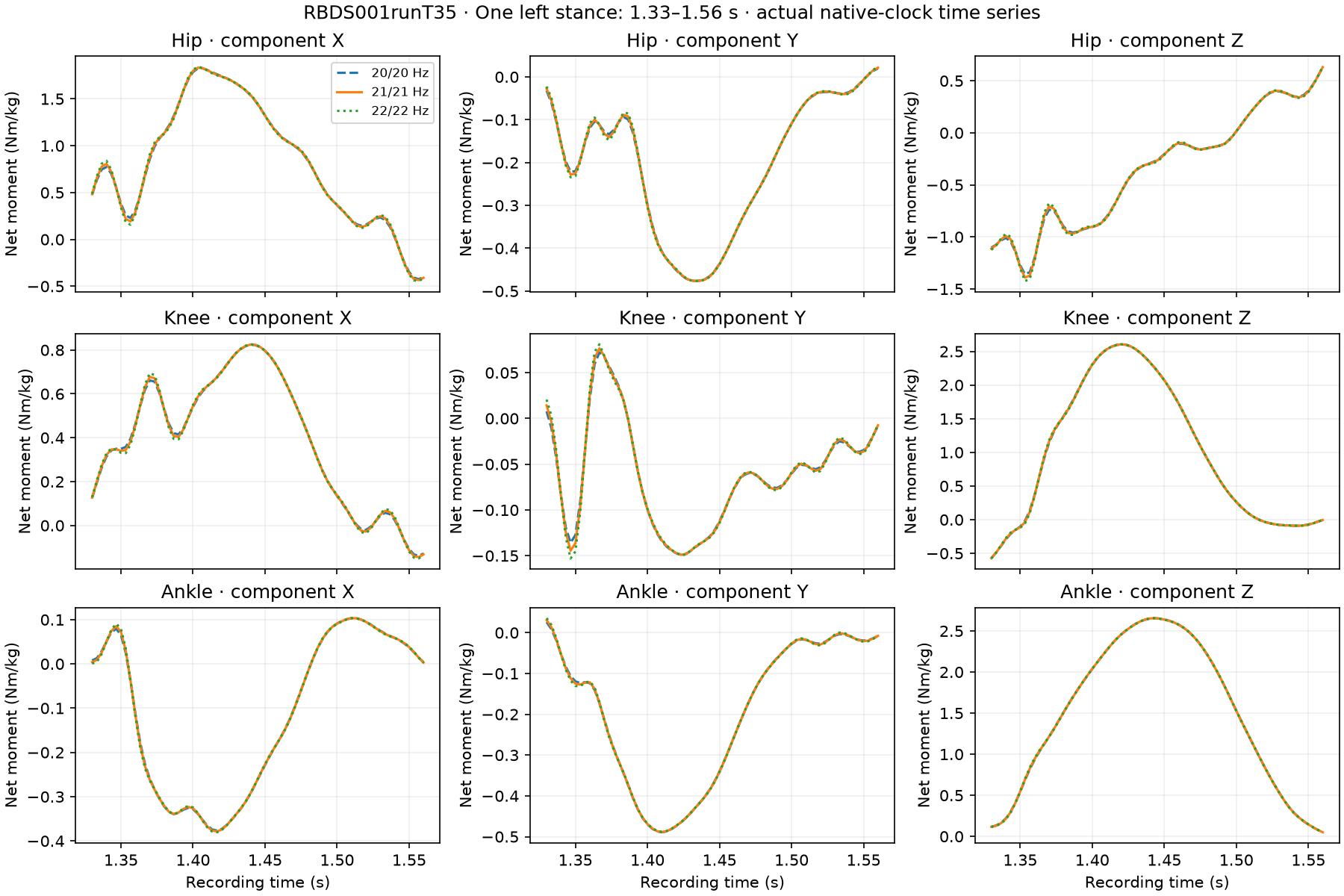
Question: how do the calculated hip, knee and ankle turning effects vary through supported stance intervals? Horizontal axis: recording time (s). Vertical axis: net joint moment per measured body mass (Nm/kg). X, Y and Z are model coordinate components; use the report’s frame definitions to interpret signs. Unsupported intervals are masked. These are model estimates, and agreement between cutoff settings cannot prove anatomical accuracy.
Public-data examples
Saved Leeds squat · concise report with figures ↗
Public General-mode example: bounded marker diagnostics of a squat. Preprocessing history is unknown; force and joint-moment recommendations are unsupported.
Saved countermovement jump · concise report with figures ↗
Public General-mode example: bilateral countermovement jump, participant 01. Unfiltered trajectories are source-reported; initial labeling and gap filling may be present. Marker diagnostics only; force and joint-moment recommendations are unsupported.
Saved Winter comparison · nine running trials
These public-data examples contain saved measurements. Select a trial to inspect its results; recommendations for your current file appear separately above.
Read the plots · fixed RBDS001runT35 example
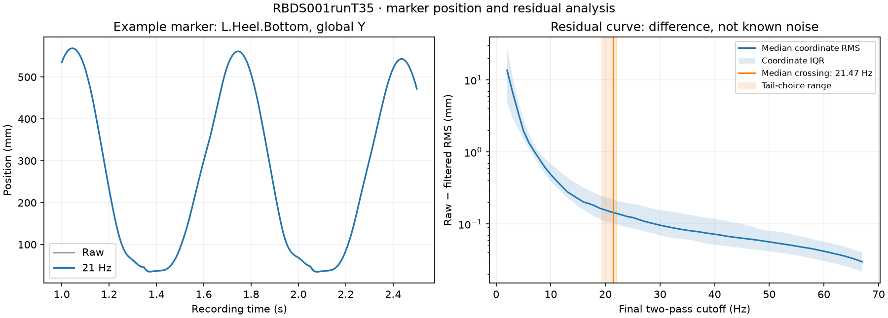
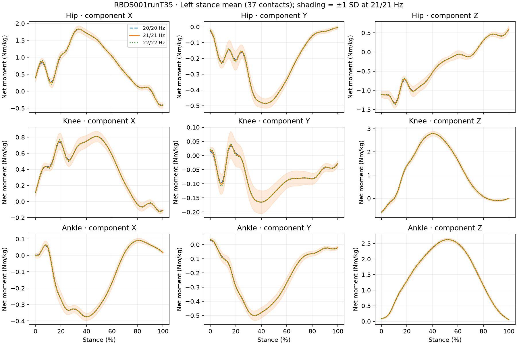
All four figures below show participant 001 running at 3.5 m/s. The recording selector changes the numerical evidence above; these figures remain this same example. Read marker filtering, force preservation and calculated moments together.
1 · Marker motion: how much movement does filtering remove?
2 · External force: compare raw force with 20, 21 and 22 Hz filtering
3 · Calculated joint moments: the net turning effect at hip, knee and ankle
4 · Average left stance: compare the shape at the same percentage of contact
ACF three-measure checks for this example
The residual-autocorrelation example issued no strict three-measure pair for RBDS001runT35: its marker ranking was unstable and its shortlisted moment comparisons exceeded declared sensitivity limits. Its separate diagnostic calculation used 22/22 Hz. That is a different method and calculation from the saved Winter 21/21 Hz experiment shown above. A provisional starting recommendation can be shown while strict eligibility remains unestablished.
Why a cutoff changes the answer
Methods & equations ↗1 · Motion
Marker positions estimate segment motion. Velocity and acceleration require differentiation, which amplifies high-frequency fluctuations. Some fluctuations may be noise; some may be real movement.
2 · External forces
Force platforms measure ground reactions. A low cutoff can suppress an impact peak; a high cutoff can retain noise or platform resonance. Preserving a raw peak therefore does not prove the true force was preserved.
3 · Joint moments
Inverse dynamics combines motion, segment mass properties and external forces through force and moment balance. Filtering either input can change the calculated net joint moments.
The practical question: which tested setting survives explicit checks, and which assumptions still need validation? Matching motion and force cutoffs is a tested starting convention here, not a universal physical requirement.
What “cutoff” means in this tool
The pipeline applies an offline, zero-phase Butterworth low-pass filter, order 2 per pass, forward and backward in second-order sections with odd padding. The named cutoff is the final two-pass −3 dB frequency (about 0.707 amplitude), corrected using the exact digital frequency relation. It is not the single-pass design frequency. Forward/backward filtering gives a fourth-order asymptotic magnitude roll-off; it is not a causal fourth-order real-time filter.
Signals are filtered at their native rates before contact summaries. Candidates at or above each signal’s Nyquist frequency (half its sample rate) are excluded. The report records coefficients, padding and comparison supports. Residual ranking trims 1 s at each recording end; signal screens declare their own guards, and moment results use 0.5 s guards at supported segment boundaries. Check the exported supports: the three checks need not retain the same number of contacts.
How the separate automatic check works
Methods & equations ↗This strict eligibility check belongs to the current-run ACF workflow. The live Winter estimate is a separate displacement-based starting setting. Its engineering limits can flag a pair for review without establishing that it is inaccurate. Automatic mode considers the first three residual-ranked marker cutoffs, retaining only those with force evidence. A pair uses the same cutoff for motion and force. Mass, height and static calibration are optional for signal screening. Without moment calculation, the conclusion reports the available provisional marker-and-force pair (or a marker-only diagnostic). With moment calculation, it issues a strict three-measure pair only when all required evidence is complete and the rules below pass.
- Marker evidence must be stable and interior. Rank raw-minus-filtered residuals by the median across valid marker coordinates of mean squared nonzero-lag autocorrelation (ACF): lower scores are preferred under a noise-like residual assumption. The primary score uses the full interior and a 0.1 s lag window; stability repeats the temporal halves and 0.05, 0.1 and 0.2 s lag windows. The winning frequency must stay unchanged across the tested windows and lag choices and must not lie on the evaluated grid boundary. This is a Challis-inspired adaptation, not an exact replication. The top-three shortlist is an engineering choice, not a confidence interval.
- Preserve recorded force features. At least 2 complete interior force contacts are required. Across all retained contacts, worst absolute peak change must be ≤5% and worst absolute impulse change ≤2% relative to unfiltered force by default. Both must pass; you may change these force limits during review.
- Check joint-moment sensitivity on common support. Every shortlisted candidate needs a complete assessment on identical fixed, side-assigned contacts: at least 2 complete contacts and at least 3 common matched pairs spanning 5 Hz or more. Against every other compared pair, worst per-contact/joint/component RMS difference must be ≤0.02 Nm/kg and worst absolute positive/negative extrema difference ≤0.05 Nm/kg.
If eligible: choose the highest residual-ranked candidate that passes both force and moment limits. No moment-magnitude or smoothness minimization occurs. If evidence is incomplete, the marker check fails, or no candidate passes both force and moment limits: issue no three-measure pair. A separate diagnostic starting pair may still be available for inspection.
Diagnostic fallback and supported model protocol
The separate marker/force diagnostic prefers the highest residual-ranked matched candidate in the top-three pool passing both force limits. If none passes, it retains the highest-ranked common candidate and reports the failures. Fewer than two force contacts leaves only a marker diagnostic. This fallback cannot become a three-measure recommendation merely because a moment plot was calculated.
Custom uploads can select a supported joint-moment model:
- Fukuchi physical-marker model: map 30 dynamic roles and all 42 static roles, including the additional anatomical landmarks. Confirm the prescribed pelvis, thigh, shank, heel and foot placements in Fukuchi et al., Table 1 and Figure 1.
- CAST configurable-cluster model: map 18 static anatomical roles and declare seven tracking groups: pelvis, bilateral thighs, shanks and feet. Each group needs at least three non-collinear measured markers, with every selected tracking marker matched in the static trial. This adapter reports net internal moments in each distal anatomical XYZ frame using its declared joint-centre and inertial assumptions.
Both models require the same participant and marker placement, measured mass and height, and one platform with mm markers and N/Nmm/mm force units in an unchanged positive-global-Y world frame and origin. Check hardware synchronization and every force-to-foot assignment.
Plug-in Gait / CGM1 and CGM2.3 use the pinned pyCGM2 calibration and lower-limb kinetics when its runtime is available. CGM2.3 includes OpenSim inverse kinematics. These workflows require measured CGM anthropometry, a matching static trial, positive global Z up and whole-record force-platform assignments. The fixed upstream 6 Hz COM filter and clinical moment projection remain in the provenance. Renaming markers does not establish equivalence between models.
Marker models, calibration and reporting conventions ↗
Signal-screen selections and contact thresholds do not redefine the moment model’s fixed calibration or contacts. Explicit same-frame rigid-cluster marker reconstruction may be used by the moment workflow; rejected estimates, gaps, exclusions and quality checks remain in its provenance.
The 5%/2% force limits, 0.02/0.05 Nm/kg moment limits, top-three pool and comparison-span requirements are this prototype’s engineering review rules. They are not accuracy limits validated by the cited literature.
How to interpret your conclusion
Conclusion rules — how to read this result
- The final provisional three-measure selection ranks the residual-shortlisted matched candidates and requires stable interior marker evidence plus unchanged force and moment-sensitivity limits. Incomplete or failing evidence produces no three-measure pair. A marker/force diagnostic starting pair is reported separately. This heuristic is not a validated moment optimum; it assumes noise-like residuals and matched bandwidth as a starting convention.
- A force shortlist needs at least 2 complete interior contacts. Relative to the unfiltered recording, across all retained contacts, worst absolute peak change must be ≤ the entered peak limit AND worst absolute impulse change must be ≤ the entered impulse limit (defaults: 5% and 2%, adjustable). This describes recorded features, not force accuracy.
- Marker residuals and smoothness alone cannot choose an optimal cutoff. Tested cutoffs stay below native Nyquist, with the declared edge guard applied.
- With a supported participant calibration, the app calculates moments across the declared candidate set. Marker evidence, force preservation and fixed-contact moment sensitivity jointly determine whether a provisional pair is eligible. If evidence is unstable, incomplete or fails the declared limits, no three-measure pair is issued. Reconstructed markers and excluded contacts are reported.
- A final pair needs explicit moment comparisons and justified model, noise, and outcome evidence; stable curves alone are insufficient. This app identifies no validated optimum. Your confirmations are workflow assertions, not independent validation.
Full conclusion and analysis limits
No recording-specific conclusion yet. Default force limits are 5% peak and 2% impulse; these can be changed during review.
Scientific context and publication use
Challis (1999) motivates residual-autocorrelation reasoning. Mai & Willwacher (2019), Bisseling & Hof (2006) and Kristianslund et al. (2012) discuss filtering and inverse-dynamics sensitivity. These primary papers support investigating the problem; this tool does not reproduce their methods exactly or validate its own thresholds through them.
What to report in a study
Help readers understand what data you used, which settings you chose, and why. You do not need to explain every calculation in the main text.
- Describe your recording. State the movement, participants and equipment. Explain where the markers were placed and how the force measurements were checked. For joint moments, also describe the body model and participant measurements used.
- Give both cutoff frequencies. Report the marker setting and the force setting separately, in Hz. Explain whether you chose them yourself or used the app’s provisional suggestion. A lower cutoff removes more rapid changes, which can include both noise and real movement.
- Explain why you chose them. Summarize the marker analysis, changes in force peaks and impulse (force accumulated over a contact), and changes in joint moments when you tried other settings. Include the range of plausible settings and any warnings.
- Say how much usable data remained. Give the number of contacts used. Mention missing markers, estimated marker positions and any sections left out of the analysis.
- Save the supporting results. Keep the report, figures, data tables and settings files. These let another researcher check your reasoning and repeat the analysis.
“The result changes little when I change the cutoff” describes sensitivity. “The result is close to the true value” describes accuracy and needs a suitable independent reference. A smooth curve alone does not show that a joint moment is accurate.
Technical details for a methods section or appendix
Include these with the exported files so the analysis can be reproduced:
- Measurements and model: dataset, participant calibration, marker-to-model assignments, units, coordinate axes, sampling rates and synchronization.
- Filtering: filter type and order, forward/backward processing, the definition of the reported cutoff, and all frequencies tested. This app uses a Butterworth filter of order 2 per pass, applied forward and backward; reported cutoffs refer to the final two-pass −3 dB response.
- Data handling: how contacts were detected and assigned to each foot, how much data was excluded near recording or segment boundaries, and how missing markers were reconstructed or excluded.
- Decision and limitations: the comparison limits used, how the final pair was chosen, model assumptions, and any independent validation. Identify a saved demonstration separately from your own recording’s results.
- Files to retain: the report and figures, CSV data tables, decision JSON (the machine-readable settings and results), and moment provenance (the record of inputs and calculation steps).